cone_beam_geometry¶

odl.tomo.geometry.conebeam.cone_beam_geometry(space, src_radius, det_radius, num_angles=None, short_scan=False, det_shape=None)[source]¶

Create a default fan or cone beam geometry from space.

This function is intended for simple test cases where users do not need the full flexibility of the geometries, but simply wants a geometry that works.

The geometry returned by this function has equidistant angles that lie (strictly) between 0 and either 2 * pi (full scan) or pi + fan_angle (short scan). The detector is centered around 0, and its size is chosen such that the whole space is covered with lines.

The number of angles and detector elements is chosen such that the resulting sinogram is fully sampled according to the Nyquist criterion, which in general results in a very large number of samples. In particular, a space that is not centered at the origin can result in very large detectors since the latter is always origin-centered.

Parameters

spaceDiscretizedSpace: Reconstruction space, the space of the volumetric data to be projected. Must be 2- or 3-dimensional.
src_radiusnonnegative float: Radius of the source circle. Must be larger than the radius of the smallest vertical cylinder containing space.domain, i.e., the source must be outside the volume for all rotations.
det_radiusnonnegative float: Radius of the detector circle.
short_scanbool, optional: Use the minimum required angular range [0, pi + fan_angle]. For True, the parker_weighting should be used in FBP. By default, the range [0, 2 * pi] is used.
num_anglesint, optional: Number of angles. Default: Enough to fully sample the data, see Notes.
det_shapeint or sequence of ints, optional: Number of detector pixels. Default: Enough to fully sample the data, see Notes.

Returns

geometryDivergentBeamGeometry

Projection geometry with equidistant angles and zero-centered detector as determined by sampling criteria.

If space is 2D, the result is a FanBeamGeometry.

If space is 3D, the result is a ConeBeamGeometry.

Notes

According to [NW2001], pages 75–76, a function $f : \mathbb{R}^2 \to \mathbb{R}$ that has compact support

$\| x \| > \rho \implies f(x) = 0,$

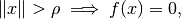
and is essentially bandlimited

$\| \xi \| > \Omega \implies \hat{f}(\xi) \approx 0,$

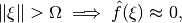
can be fully reconstructed from a fan beam ray transform with source-detector distance $r$ (assuming all detector points have the same distance to the source) if (1) the projection angles are sampled with a spacing of $\Delta \psi$ such that

$\Delta \psi \leq \frac{r + \rho}{r}\, \frac{\pi}{\rho \Omega},$

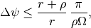
and (2) the detector is sampled with an angular interval $\Delta \alpha$ that satisfies

$\Delta \alpha \leq \frac{\pi}{r \Omega}.$

For a flat detector, the angular interval is smallest in the center of the fan and largest at the boundaries. The worst-case relation between the linear and angular sampling intervals are

$\Delta s = R \Delta \alpha, \quad R^2 = r^2 + (w / 2)^2,$

where $w$ is the width of the detector. Thus, to satisfy the angular detector condition one can choose

$\Delta s \leq \frac{\pi \sqrt{r^2 + (w / 2)^2}}{r \Omega}.$

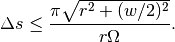
The geometry returned by this function satisfies these conditions exactly.

If the domain is 3-dimensional, a circular cone beam geometry is created with the third coordinate axis as rotation axis. This does, of course, not yield complete data, but is equivalent to the 2D fan beam case in the $z = 0$ slice. The vertical size of the detector is chosen such that it covers the object vertically with rays, using a containing cuboid $[-\rho, \rho]^2 \times [z_{\mathrm{min}}, z_{\mathrm{min}}]$ to compute the cone angle.

References

NW2001: Natterer, F and Wuebbeling, F. Mathematical Methods in Image Reconstruction. SIAM, 2001. https://dx.doi.org/10.1137/1.9780898718324

Examples

Create a fan beam geometry from a 2d space:

>>> space = odl.uniform_discr([-1, -1], [1, 1], (20, 20))
>>> geometry = cone_beam_geometry(space, src_radius=5, det_radius=5)
>>> geometry.angles.size
78
>>> geometry.detector.size
57

For a short scan geometry (from 0 to pi + fan_angle), the short_scan flag can be set, resulting in a smaller number of angles:

>>> geometry = cone_beam_geometry(space, src_radius=5, det_radius=5,
...                               short_scan=True)
>>> geometry.angles.size
46

If the source is close to the object, the detector becomes larger due to more magnification:

>>> geometry = cone_beam_geometry(space, src_radius=3, det_radius=9)
>>> geometry.angles.size
80
>>> geometry.detector.size
105